Fitting guide
This is a summary of the methods used by nanite for fitting force-distance data. Examples are given below.
Preprocessors
Prior to data analysis, a force-distance curve has to be preprocessed. One of the most important preprocessing steps is to perform a tip-sample separation which computes the correct tip position from the recorded piezo height and the cantilever deflection. Other preprocessing steps correct for offsets or smoothen the data:
preprocessor key |
description |
details |
|---|---|---|
compute_tip_position |
tip-sample separation |
|
correct_force_offset |
baseline offset correction |
|
correct_force_slope |
baseline slope correction |
|
correct_tip_offset |
contact point estimation |
|
correct_split_approach_retract |
segment discovery |
|
smooth_height |
monotonic height data |
Several methods for estimating the point of contact (POC) are implemented in nanite:
POC method |
description |
details |
|---|---|---|
deviation_from_baseline |
Deviation from baseline |
|
fit_constant_line |
Piecewise fit with constant and line |
|
fit_constant_polynomial |
Piecewise fit with constant and polynomial |
|
fit_line_polynomial |
Piecewise fit with line and polynomial |
|
frechet_direct_path |
Fréchet distance to direct path |
|
gradient_zero_crossing |
Gradient zero-crossing of indentation part |
Models
Nanite comes with a predefined set of model functions that are identified (in scripting as well as in the command line interface) via their model keys.
model key |
description |
details |
|---|---|---|
hertz_cone |
conical indenter (Hertz) |
|
hertz_para |
parabolic indenter (Hertz) |
|
hertz_pyr3s |
pyramidal indenter, three-sided (Hertz) |
|
power_layer_clifford_2009 |
elastic layer power law (Clifford 2009) |
|
sneddon_spher |
spherical indenter (Sneddon) |
|
sneddon_spher_approx |
spherical indenter (Sneddon, truncated power series) |
These model functions can be used to fit experimental force-distance data that have been preprocessed as described above.
Parameters
Besides the modeling parameters (e.g. Young’s modulus or contact point),
nanite allows to define an extensive set of fitting options, that
are described in more detail in nanite.fit.IndentationFitter.
parameter |
description |
|---|---|
model_key |
Key of the model function used |
optimal_fit_edelta |
Plateau search for Young’s modulus |
optimal_fit_num_samples |
Number of points for plateau search |
params_initial |
Initial parameters |
preprocessing |
List of preprocessor keys |
range_type |
‘absolute’ for static range, ‘relative cp’ for dynamic range |
range_x |
Fitting range (min/max) |
segment |
Which segment to fit (‘approach’ or ‘retract’) |
weight_cp |
Suppression of residuals near contact point |
x_axis |
X-data used for fitting (defaults to ‘top position’) |
y_axis |
Y-data used for fitting (defaults to ‘force’) |
method |
Minimizer method for lmfit.minimize |
method_kws |
Additional arguments (fit_kws) for the underlying scipy minimizer function |
Geometrical correction factor
The basic models implemented in nanite are all single-contact models, which means that they assume there is only one indentation taking place during a measurement. In an AFM experiment, this holds true for e.g. measuring a flat hydrogel with a spherical AFM tip. However, many experiments require a two-contact model. A prominent example is the indentation of an elastic sphere between two parallel plates (e.g. a round cell on a glass cover slip indented by a wedged cantilever). Here, the top and bottom indentation of the sphere contribute to the overall indentation. However, the forces required to indent either side of the sphere are identical to the force in the single-contact version of the problem (where the elastic sphere is the cantilever). For instance, you need twice the force to squeeze a ball between your hands compared to when you squeeze it against a wall, but the overall indentation stays the same (Newton’s third law). Thus, when you use a single-contact model in a two-contact problem, you have to be aware of the fact that the actual indentation may be larger. For the simple example of parallel-plate compression, the actual indentation is doubled. Thus, to be able to apply the single-contact model fit, we have to multiply the measured indentation by a factor of \(k=0.5\).
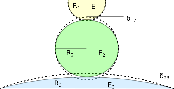
Fig. 1 Two-contact geometry for three elastic spheres.
Let’s take a look at the more general geometric problem (still neglecting adhesion forces and gravity). Let’s assume whe have three spheres with Young’s modul \(E_1\), \(E_2\), \(E_3\) and radii \(R_1\), \(R_2\), \(R_3\) (see figure Fig. 1). This is a two-contact problem. For each of the contact areas we can write down the Hertz model for the single-contact problem. The overall indentation is \(\delta = \delta_{12} + \delta_{23}\) with
and
From here, we can start simplifying. Let’s say the indenter and the substrate are comparatively stiff (\(E_1 = E_3 >> E_2\)) and the substrate is flat (\(R_3 \rightarrow \inf\)). Then we get
Thus, the overall indentation becomes
Finally, we arrive at
The parameter \(k\) is the geometrical correction factor. For an indenter with \(R_1 = 2.5\,\text{µm}\) and a cell with \(R_2 = 7.5\,\text{µm}\), the geometrical correction factor computes to \(k=0.6135\). Note that during fitting with the single-contact model, you now have to set the radius to the effective radius \(R_{12}=1.875\,\text{µm}\).
For a more general description of this problem, please have a look at [GMP+14].
Workflow
There are two ways to fit force-distance curves with nanite: via the command line interface (CLI) or via Python scripting. The CLI does not require programming knowledge while Python-scripting allows fine-tuning and straight-forward automation.
Command-line usage
First, set up a fitting profile by running (e.g. in a command prompt on Windows).
nanite-setup-profile
This program will ask you to specify preprocessors, model parameters, and other fitting parameters. Simply enter the values via the keyboard and hit enter to let them be acknowledged. If you want to use the default values, simply hit enter without typing anything. A typical output will look like this:
Define preprocessing:
  1: compute_tip_position
  2: correct_force_offset
  3: correct_split_approach_retract
  4: correct_tip_offset
  5: smooth_height
(currently '1,2,4'):

Select model number:
  1: hertz_cone
  2: hertz_para
  3: hertz_pyr3s
  4: sneddon_spher
  5: sneddon_spher_approx
(currently '5'):

Set fit parameters:
- initial value for E [Pa] (currently '3000.0'): 50
  vary E (currently 'True'):
- initial value for R [m] (currently '1e-5'): 18.64e-06
  vary R (currently 'False'):
- initial value for nu (currently '0.5'):
  vary nu (currently 'False'):
- initial value for contact_point [m] (currently '0.0'):
  vary contact_point (currently 'True'):
- initial value for baseline [N] (currently '0.0'):
  vary baseline (currently 'False'):

Select range type (absolute or relative):
(currently 'absolute'):

Select fitting interval:
left [µm] (currently '0.0'):
right [µm] (currently '0.0'):

Suppress residuals near contact point:
size [µm] (currently '0.5'): 2

Select training set:
training set (path or name) (currently 'zef18'):

Select rating regressor:
  1: AdaBoost
  2: Decision Tree
  3: Extra Trees
  4: Gradient Tree Boosting
  5: Random Forest
  6: SVR (RBF kernel)
  7: SVR (linear kernel)
(currently '3'):

Done. You may edit all parameters in '/home/user/.config/nanite/cli_profile.cfg'.
In this example, the only modifications of the default values are
the initial value of the Young’s modulus (50 Pa),
the value for the tip radius (18.64 µm),
and the suppression of residuals near the contact point with a ±2 µm interval.
When nanite-setup-profile is run again, it will use the values from the
previous run as default values. The training set and rating regressor
options are discussed in the rating workflow.
Finally, to perform the actual fitting, use the command-line script
nanite-fit data_path output_path
This command will recursively search the input folder data_path for
data files, fit the data with the parameters in the profile, and write the
statistics (statistics.tsv) and visualizations of the fits
(multi-page TIFF file plots.tif, open with Fiji
or the Windows Photo Viewer) to the directory output_path.
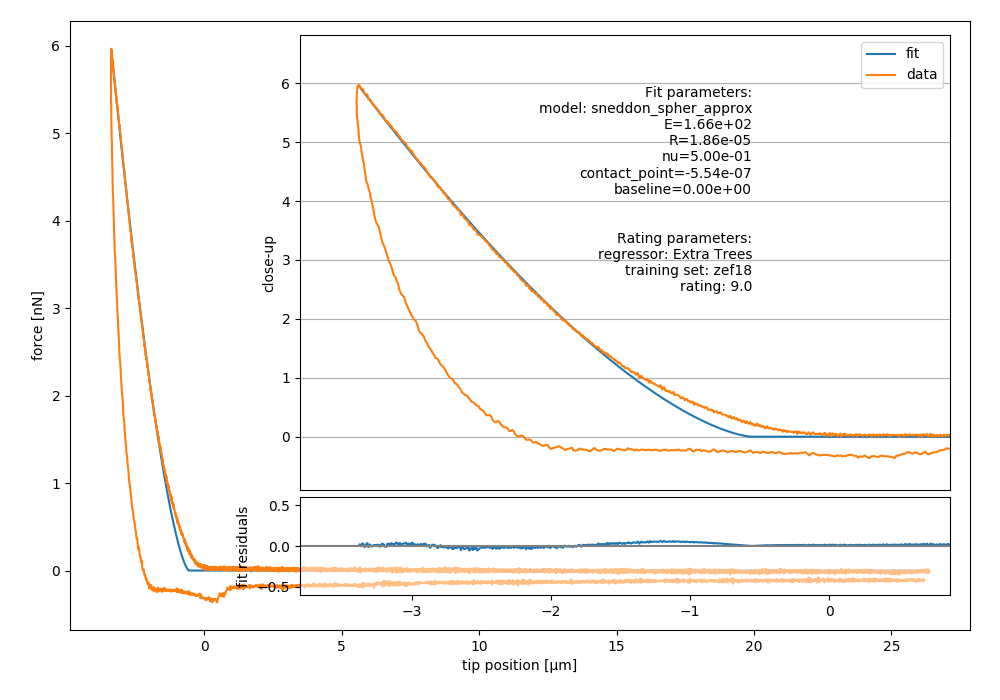
Fig. 2 Example image generated with nanite-fit. Note that the dataset
is already rated with the default method “Extra Trees” and the
default training set label “zef18”. See Rating workflow for more
information on rating.
Scripting usage
Using nanite in a Python script for data fitting is straight forward.
First, load the data; group is an instance of
nanite.IndentationGroup:
In [1]: import nanite

In [2]: group = nanite.load_group("data/force-save-example.jpk-force")
Second, obtain the first nanite.Indentation instance and apply
the preprocessing:
In [3]: idnt = group[0]

In [4]: idnt.apply_preprocessing(["compute_tip_position",
   ...:                           "correct_force_offset",
   ...:                           "correct_tip_offset"])
   ...:
Now, setup the model parameters:
In [5]: idnt.fit_properties["model_key"] = "sneddon_spher"

In [6]: params = idnt.get_initial_fit_parameters()

In [7]: params["E"].value = 50

In [8]: params["R"].value = 18.64e-06

In [9]: params.pretty_print()
Name              Value      Min      Max   Stderr     Vary     Expr Brute_Step
E                    50        0      inf     None     True     None     None
R              1.864e-05        0      inf     None    False     None     None
baseline              0     -inf      inf     None     True     None     None
contact_point         0     -inf      inf     None     True     None     None
nu                  0.5        0      0.5     None    False     None     None
Finally, fit the model:
In [10]: idnt.fit_model(model_key="sneddon_spher", params_initial=params, weight_cp=2e-6)

In [11]: idnt.fit_properties["params_fitted"].pretty_print()
Name              Value      Min      Max   Stderr     Vary     Expr Brute_Step
E                 165.8        0      inf   0.1805     True     None     None
R              1.864e-05        0      inf        0    False     None     None
baseline       -6.089e-13     -inf      inf 2.318e-13     True     None     None
contact_point  -5.54e-07     -inf      inf 1.624e-09     True     None     None
nu                  0.5        0      0.5        0    False     None     None
The fitting results are identical to those shown in figure 2 above.
Note that, amongst other things, preprocessing can also be specified
directly in the
fit_model function.